Learning
Given an observation sequence ![]() and the set of possible states in the HMM, learn the HMM parameters
and the set of possible states in the HMM, learn the HMM parameters ![]() and
and ![]() .
.
The standard algorithm for HMM training is the Forward-Backward, or Baum-Welch algorithm. It is an iterative algorithm, computing an initial estimate for the probabilities, then using those estimates to computing a better estimate, and so on, iteratively improving the probabilities that it learns.
Backward Probability
The backward probability ![]() is the probability of seeing the observations from time
is the probability of seeing the observations from time ![]() to the end, given that we are in state
to the end, given that we are in state ![]() at time
at time ![]() (and given the HMM
(and given the HMM ![]() ):
):
The state at ![]() can be any of N states.
can be any of N states.
Observations ![]() are independent of
are independent of ![]() and
and ![]() .
.
Observation ![]() is independent of
is independent of ![]() .
.
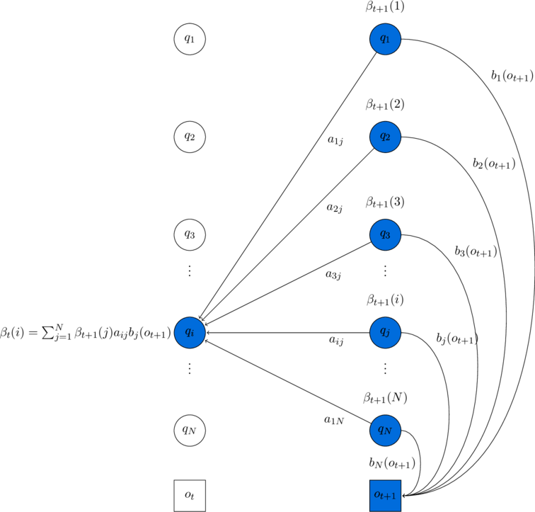
Visualization
The computation of ![]() by summing all the successive values
by summing all the successive values ![]() weighted by their transition probabilities
weighted by their transition probabilities ![]() and their observation probabilities
and their observation probabilities ![]() . Hidden states are in circles, observations in squares. Shaded nodes are included in the probability computation for
. Hidden states are in circles, observations in squares. Shaded nodes are included in the probability computation for ![]() .
.
Initialization
Recursion
Termination
Probability 
Define the probability ![]() as the probability of being in state
as the probability of being in state ![]() at time
at time ![]() and state
and state ![]() at time
at time ![]() , given the observation sequence and the model.
, given the observation sequence and the model.
The observation ![]() is defined as
is defined as ![]()
The observation ![]() , emitted at state
, emitted at state ![]() , will only depend on the state
, will only depend on the state ![]() . Simplifying
. Simplifying
The observations ![]() to
to ![]() and the state
and the state ![]() do not depend on any observation from
do not depend on any observation from ![]() to
to ![]() . Simplifying
. Simplifying
The observations ![]() to
to ![]() do not depend on the state
do not depend on the state ![]() . Simplifying
. Simplifying
Visualization
\clearpage
Computation of the joint probability of being in state ![]() at time
at time ![]() and state
and state ![]() at time
at time ![]() . The figure shows the various probabilities that need to be combined to produce
. The figure shows the various probabilities that need to be combined to produce ![]() : the
: the ![]() and
and ![]() probabilities, the transition probability
probabilities, the transition probability ![]() and the observation probability
and the observation probability ![]() . Hidden states are in circles, observations in squares. Shaded nodes are included in the probability computation for
. Hidden states are in circles, observations in squares. Shaded nodes are included in the probability computation for ![]() .
.
The probability of the observation given the model is simply the forward probability of the whole utterance (or alternatively, the backward probability of the whole utterance):
The state ![]() can be any of
can be any of ![]() possible states.
possible states.
Observations ![]() do not depend on observations
do not depend on observations ![]()
Define the probability ![]() as the probability of being in state
as the probability of being in state ![]() at time
at time ![]() .
.
Observations ![]() do not depend on observations
do not depend on observations ![]()
Estimate 
Estimate 
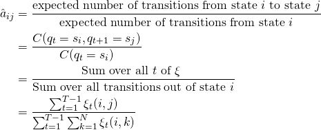
The forward-backward algorithm has two steps: the expectation step, or E-step, and the maximization step, or M-step.
In the E-step, the expected state occupancy count ![]() and the expected state transition count
and the expected state transition count ![]() from the earlier
from the earlier ![]() and
and ![]() probabilities are computed.
probabilities are computed.
In the M-step, ![]() and
and ![]() are used to recompute new
are used to recompute new ![]() and
and ![]() probabilities.
probabilities.


