The Gaussian Distribution

The Gaussian (Normal) distribution is a probability density function specified by two parameters – mean $\mu$ and variance $\sigma^2$ . If a single variable, say $x$ , is normally distributed the density function is abbreviated as $p(x) \sim \mathcal{N}(\mu, \sigma^2)$ . The square root of the variance is called the standard deviation $\sigma$ . The inverse of the variance is called the precision $\beta = \frac{1}{\sigma^2}$ . The function is defined as follows

$\begin{equation*} p(x) = \frac{1}{\sqrt{2 \pi } \sigma} \text{exp}\Bigg[\frac{1}{2} \Bigg( \frac{x - \mu}{\sigma} \Bigg)^2 \Bigg] \end{equation*}$

Visualization

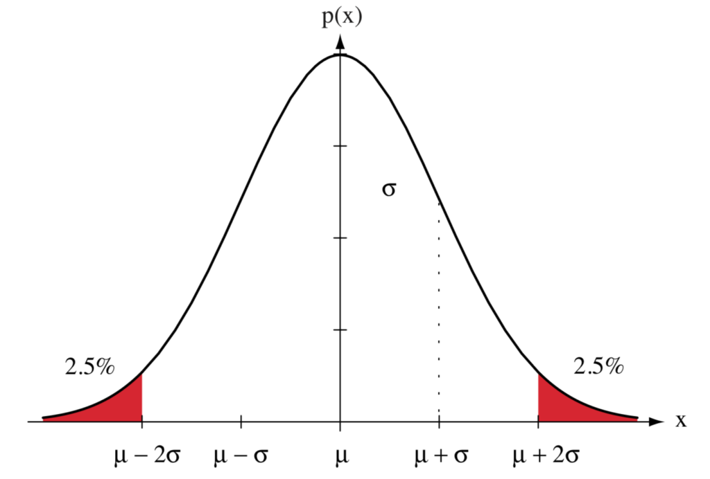
95% of the area under the Gaussian distribution curve lies within 2 standard deviation units about the mean.

Positive

Because of the exponential term, the above density function is always positive.

$\begin{equation*} p(x) > 0 \end{equation*}$

Maximum

The peak of the Gaussian distribution occurs when $x = \mu$

$\begin{equation*}p(\mu) = \frac{1}{\sqrt{2 \pi} \sigma} \end{equation*}$

Normalized

Over the entire feature space, the density function integrates to 1, thus making it a valid probability distribution.

Define

$\begin{equation*} a = \frac{x- \mu}{\sqrt{2} \sigma} \quad \quad dx = da (\sqrt{2} \sigma) \end{equation*}$

Substituting and using the fact that $e^{-a^2}$ is an even function

$\begin{equation*} \int_{-\infty}^{\infty} p(x) dx \end{equation*}$

$\begin{equation*} = \int_{-\infty}^{\infty} \frac{1}{\sqrt{2 \pi } \sigma} \text{exp} \Bigg[ \frac{1}{2} \Bigg( \frac{x - \mu}{\sigma} \Bigg)^2 \Bigg] dx\end{equation*}$

$\begin{equation*} = \frac{1}{\sqrt{\pi }} \int_{-\infty}^{\infty} e^{-a^2} da = \frac{2}{\sqrt{\pi }} \int_{0}^{\infty} e^{-a^2} da \end{equation*}$

There are several tricks to solve this definite Gaussian integral by using the following property

$\begin{equation*} \Bigg( \int_{0}^{\infty} e^{-a^2} da \Bigg)^2 \end{equation*}$

$\begin{equation*} = \int_{0}^{\infty} e^{-a^2} da \int_{0}^{\infty} e^{-b^2} db \end{equation*}$

$\begin{equation*} = \int_{0}^{\infty} \int_{0}^{\infty} e^{-(a^2 + b^2)} da \, db \end{equation*}$

Define

$\begin{equation*} b = as \quad \quad db = a \, ds \end{equation*}$

$\begin{equation*} \frac{2}{\sqrt{\pi }} \int_{0}^{\infty} e^{-a^2} da \end{equation*}$

$\begin{equation*} = \frac{2}{\sqrt{\pi }} \Bigg[ \int_{0}^{\infty} \int_{0}^{\infty} e^{-(a^2 + b^2)} da \, db \Bigg]^{\frac{1}{2}} \end{equation*}$

$\begin{equation*} = \frac{2}{\sqrt{\pi }} \Bigg[ \int_0^\infty \left( \int_0^\infty e^{-(a^2 + b^2)} \, db \right) \, da \Bigg ]^{\frac{1}{2}} \end{equation*}$

$\begin{equation*} = \frac{2}{\sqrt{\pi }} \Bigg[ \int_0^\infty \left( \int_0^\infty e^{-a^2(1+s^2)} a\,ds \right) \, da \Bigg ]^{\frac{1}{2}} \end{equation*}$

$\begin{equation*} = \frac{2}{\sqrt{\pi }} \Bigg[ \int_0^\infty \left( \int_0^\infty e^{-a^2(1 + s^2)} a \, da \right) \, ds \Bigg ]^{\frac{1}{2}} \end{equation*}$

$\begin{equation*} = \frac{2}{\sqrt{\pi }} \Bigg[ \int_0^\infty \left[ \frac{1}{-2(1+s^2)} e^{-a^2(1+s^2)} \right]_{a=0}^{a=\infty} \, ds \Bigg ]^{\frac{1}{2}} \end{equation*}$

$\begin{equation*} = \frac{2}{\sqrt{\pi }} \Bigg[ \frac{1}{2} \int_0^\infty \frac{ds}{1+s^2} \Bigg ]^{\frac{1}{2}} \end{equation*}$

$\begin{equation*} = \frac{2}{\sqrt{\pi }} \Bigg[ \frac{1}{2} \Big [ \tan^{-1} s \Big ]_0^\infty \Bigg ]^{\frac{1}{2}} \end{equation*}$

$\begin{equation*} = \frac{2}{\sqrt{\pi }} \Bigg[ \frac{\pi}{4} \Bigg ]^{\frac{1}{2}} = 1 \end{equation*}$

Mean

The mean is defined by the expected value of the input variable over the entire feature space

$\begin{equation*} \mathcal{E}[x] = \int_{-\infty}^{\infty} x p(x) \, dx \end{equation*}$

$\begin{equation*} = \int_{-\infty}^{\infty} x \frac{1}{\sqrt{2 \pi } \sigma} \text{exp} \Bigg[ - \frac{1}{2} \Bigg( \frac{x - \mu}{\sigma} \Bigg)^2 \Bigg] dx \end{equation*}$

Define

$\begin{equation*} a = x - \mu \quad \quad da = dx \end{equation*}$

Substituting

$\begin{equation*} \int_{-\infty}^{\infty} (a + \mu) \frac{1}{\sqrt{2 \pi } \sigma} \text{exp} \Bigg[ - \frac{1}{2} \Bigg( \frac{a}{\sigma} \Bigg)^2 \Bigg] da\end{equation*}$

$\begin{equation*} = \int_{-\infty}^{\infty} a \frac{1}{\sqrt{2 \pi } \sigma} \text{exp} \Bigg[ - \frac{1}{2} \Bigg( \frac{a}{\sigma} \Bigg)^2 \Bigg] da \end{equation*}$

$\begin{equation*} + \mu \int_{-\infty}^{\infty} \frac{1}{\sqrt{2 \pi } \sigma} \text{exp} \Bigg[ - \frac{1}{2} \Bigg( \frac{a}{\sigma} \Bigg)^2 \Bigg] da \end{equation*}$

The first term integrates to 0 because the integrand is an odd function and the integral is over the entire feature space. The integrand in the second term is another (zero-mean) gaussian distribution and as such integrates to 1 over the entire feature space. Thus

$\begin{equation*}\mathcal{E}[x]=\mu\end{equation*}$

Variance

The variance is defined by the expected squared deviation of the input variable from the mean over the entire feature space.

$\begin{equation*} \mathcal{E}[(x - \mu)^2] = \int_{-\infty}^{\infty} (x - \mu)^2 p(x) \, dx \end{equation*}$

$\begin{equation*} = \int_{-\infty}^{\infty} (x - \mu)^2 \frac{1}{\sqrt{2 \pi } \sigma} \text{exp} \Bigg[ - \frac{1}{2} \Bigg( \frac{x - \mu}{\sigma} \Bigg)^2 \Bigg] dx \end{equation*}$

Define

$\begin{equation*} a = \frac{x - \mu}{\sqrt{2} \sigma} \quad \quad dx = \sqrt{2} \sigma \, da \end{equation*}$

Substituting

$\begin{equation*} \int_{-\infty}^{\infty} 2 \sigma^2 a^2 \frac{1}{\sqrt{2 \pi } \sigma} e^{-a^2} \sqrt{2} \sigma \, da \end{equation*}$

$\begin{equation*} = \frac{2 \sigma^2}{\sqrt{\pi}} \int_{-\infty}^{\infty} a \cdot a e^{-a^2} \, da \end{equation*}$

Using integration by parts

$\begin{equation*} \mathcal{E}[x] = \frac{2 \sigma^2}{\sqrt{\pi}} \Bigg( \Bigg[ a \frac{-1}{2} e^{-a^2} \Bigg]_{-\infty}^{\infty} - \int_{-\infty}^{\infty} \frac{-1}{2} e^{-a^2} da \Bigg) \end{equation*}$

The first term integrates to 0 because the integrand is an odd function and the integral is over the entire feature space. The second term is the Gaussian integral which evaluates to $\sqrt{\pi}$ . Thus

$\begin{equation*} \mathcal{E}[x] = \frac{2 \sigma^2}{\sqrt{\pi}} \frac{\sqrt{\pi}}{2} = \sigma^2 \end{equation*}$

The Beard Sage

Visualization

Positive

Maximum

Normalized

Mean

Variance

References

Leave a Reply Cancel reply