Gradient Descent for a Single Artificial Neuron

This article explores the gradient descent algorithm for a single artificial neuron. The activation function is set to the logistic function.

Logistic Function

The logistic function is the most common kind of sigmoid function. It is defined as follows

$\begin{equation*} \sigma(u) = \frac{1}{1 + e^{-u}} \end{equation*}$

Properties

The logistic function has two primary good properties

The output $y$ is always between $0$ and $1$ .
Unlike a unit step function, $\sigma(u)$ is smooth and differentiable, making the derivation of update equation very easy.

$\sigma(-u) = 1 - \sigma(u)$

$\begin{align*} 1 - \sigma(u) &= 1 - \frac{1}{1 + e^{-u}} \\ &= \frac{e^{-u}}{1 + e^{-u}} \\ &= \frac{1}{\frac{1}{e^{-u}} + 1} \\ &= \frac{1}{1 + e^{u}} \\ &= \sigma(-u) \qed \\ \end{align*}$

$\frac{d\sigma(u)}{du} = \sigma(u)\sigma(-u)$

$\begin{align*} \frac{d\sigma(u)}{du} &= \frac{d}{du} \Big(\frac{1}{1 + e^{-u}}\Big) \\ &= \frac{d}{du} \Big((1 + e^{-u})^{-1}\Big) \\ &= -(1 + e^{-u})^{-2} \frac{d}{du} (1 + e^{-u}) \\ &= -(1 + e^{-u})^{-2}e^{-u} \frac{d}{du} (-u) \\ &= (1 + e^{-u})^{-2}e^{-u} \\ &= \frac{1}{1 + e^{-u}}\frac{e^{-u}}{1 + e^{-u}} \\ &= \frac{1}{1 + e^{-u}}\frac{1}{e^{u} + 1} \\ &= \sigma(u)\sigma(-u) \qed \end{align*}$

Single Artificial Neuron

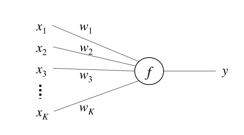
Notations

${x_1, \cdots ,x_K}$ are input values
${w_1, \cdots ,w_K}$ are weights
$y$ is a scalar output
$f$ is the activation function (also called decision/transfer function)
$t$ is the label (gold standard)
$\eta$ is is the learning rate ( $\eta > 0$ )

The unit works in the following way

$\begin{equation*} y = f(u) \end{equation*}$

where $u$ is a scalar number, which is the net input of the neuron.

$\begin{equation*} u = \sum_{i=0}^kw_ix_i \end{equation*}$

In vector notation

$\begin{equation*} u = \boldsymbol{w}^T\boldsymbol{X} \end{equation*}$

To include a bias term, simply add an input dimension (e.g., $x_0$ ) that is constant $1$ .

The error function (the training objective) is defined as

$\begin{equation*} E = \frac{1}{2}(t - y)^2 \end{equation*}$

Use stochastic gradient descent as the learning algorithm of this model – take the derivative of $E$ with regard to $w_i$

$\begin{align*} \frac{\partial E}{\partial w_i} &= \frac{\partial E}{\partial y}\cdot\frac{\partial y}{\partial u}\cdot\frac{\partial u}{\partial w_i} \\ \frac{\partial E}{\partial y} &= \frac{\partial}{\partial y}\Big(\frac{1}{2}(t - y)^2\Big) = (y - t) \\ \frac{\partial y}{\partial u} &= \frac{\partial}{\partial u}\sigma(u) = \sigma(u)\sigma(-u) = \sigma(u)(1 - \sigma(u)) = y(1 - y) \\ \frac{\partial u}{\partial w_i} &= \frac{\partial}{\partial w_i}\Big(\sum_{i=0}^kw_ix_i\Big) = x_i \\ \end{align*}$

Thus,

$\begin{equation*} \frac{\partial E}{\partial w_i} = (y-t) \cdot y(1-y) \cdot x_i \end{equation*}$

Once the derivative is computed, simply apply stochastic gradient descent for all samples

$\begin{equation*} \boldsymbol{w}^{(new)} =\boldsymbol{w}^{(old)} - \eta \cdot (y - t) \cdot y(1 - y) \cdot \boldsymbol{x} \end{equation*}$

References

https://arxiv.org/pdf/1411.2738.pdf

The Beard Sage