Inspecting word2vec Matrices

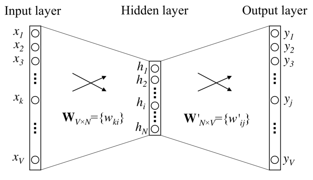
The below figure shows a representation of Continuous Bag-of-Word Model with only one word in the context. There are three layers in total. The units on adjacent layers are fully connected.

A simple CBOW model with only one word in the context.

Notations

There are $V$ words in the vocabulary.
The input layer is of size $V$ and indexed using $k$ .
The output layer is of size $V$ and indexed using $j$ .
The hidden layer is of size $N$ and indexed using $i$ .
$\mathbf{W}$ is the weight matrix connecting the input layer and the hidden layer. $\mathbf{W}$ has dimensions $V \times N$ .
An individual element in the weight matrix $\mathbf{W}$ is denoted by $w_{ki}$ . Here. $k \in \{1 \cdots V\}$ and $i \in \{1 \cdots N\}$ .
$\mathbf{W'}$ is the weight matrix connecting the hidden layer and the output layer. $\mathbf{W'}$ has dimensions $N \times V$ .
An individual element in the weight matrix $\mathbf{W'}$ is denoted by $w'_{ij}$ . Here. $i \in \{1 \cdots N\}$ and $j \in \{1 \cdots V\}$ .

Input

The input is a one-hot encoded vector. This means that for a given input context word, only one out of $V$ units, ${x_1, \cdots, x_V }$ , will be $1$ , and all other units are $0$ .

Consider an input word $x_k$ . Given a one-word context and the above one-hot encoding, $x_k = 1$ and $x_{k'} = 0$ for $k' \neq k$ .

$\begin{equation*} \mathbf{x} = \begin{bmatrix} x_{1} \\ x_{2} \\ \vdots \\ x_{k} \\ \vdots \\ x_{V} \\ \end{bmatrix}_{V\times 1} = \begin{bmatrix} 0 \\ 0 \\ \vdots \\ 1 \\ \vdots \\ 0 \\ \end{bmatrix}_{V\times 1} \end{equation*}$

Input-Hidden Weights

$\mathbf{W}$ is the weight matrix connecting the input layer and the hidden layer. $\mathbf{W}$ has dimensions $V \times N$ .

$\begin{equation*} \mathbf{W} = \begin{bmatrix} w_{11} & w_{12} & \hdots & w_{1i} & \hdots & w_{1N} \\ w_{21} & w_{22} & \hdots & w_{2i} & \hdots & w_{2N} \\ \vdots & \vdots & \ddots & \vdots & \ddots & \vdots \\ w_{k1} & w_{k2} & \hdots & w_{ki} & \hdots & w_{kN} \\ \vdots & \vdots & \ddots & \vdots & \ddots & \vdots \\ w_{V1} & w_{V2} & \hdots & w_{Vi} & \hdots & w_{VN} \\ \end{bmatrix}_{V\times N} \end{equation*}$

An individual element in the weight matrix $\mathbf{W}$ is denoted by $w_{ki}$ . Here. $k \in \{1 \cdots V\}$ and $i \in \{1 \cdots N\}$ . The transpose of the matrix is

$\begin{equation*} \mathbf{W}^T = \begin{bmatrix} w_{11} & w_{21} & \hdots & w_{k1} & \hdots & w_{V1} \\ w_{12} & w_{22} & \hdots & w_{k2} & \hdots & w_{V2} \\ \vdots & \vdots & \ddots & \vdots & \ddots & \vdots \\ w_{1i} & w_{2i} & \hdots & w_{ki} & \hdots & w_{Vi} \\ \vdots & \vdots & \ddots & \vdots & \ddots & \vdots \\ w_{1N} & w_{2N} & \hdots & w_{kN} & \hdots & w_{VN} \\ \end{bmatrix}_{N\times V} \end{equation*}$

From the network, the hidden layer is defined as follows

$\begin{equation*} \mathbf{h} = \mathbf{W}^T\mathbf{x} \end{equation*}$

$\begin{align*} \mathbf{h} & = \begin{bmatrix} w_{11} & w_{21} & \hdots & w_{k1} & \hdots & w_{V1} \\ w_{12} & w_{22} & \hdots & w_{k2} & \hdots & w_{V2} \\ \vdots & \vdots & \ddots & \vdots & \ddots & \vdots \\ w_{1i} & w_{2i} & \hdots & w_{ki} & \hdots & w_{Vi} \\ \vdots & \vdots & \ddots & \vdots & \ddots & \vdots \\ w_{1N} & w_{2N} & \hdots & w_{kN} & \hdots & w_{VN} \\ \end{bmatrix}_{N\times V} \times \begin{bmatrix} x_{1} \\ x_{2} \\ \vdots \\ x_{k} \\ \vdots \\ x_{V} \\ \end{bmatrix}_{V\times 1} \\ & = \begin{bmatrix} w_{11} & w_{21} & \hdots & w_{k1} & \hdots & w_{V1} \\ w_{12} & w_{22} & \hdots & w_{k2} & \hdots & w_{V2} \\ \vdots & \vdots & \ddots & \vdots & \ddots & \vdots \\ w_{1i} & w_{2i} & \hdots & w_{ki} & \hdots & w_{Vi} \\ \vdots & \vdots & \ddots & \vdots & \ddots & \vdots \\ w_{1N} & w_{2N} & \hdots & w_{kN} & \hdots & w_{VN} \\ \end{bmatrix}_{N\times V} \times \begin{bmatrix} 0 \\ 0 \\ \vdots \\ 1 \\ \vdots \\ 0 \\ \end{bmatrix}_{V\times 1} \\ & = \begin{bmatrix} w_{k1} \\ w_{k2} \\ \vdots \\ w_{ki} \\ \vdots \\ w_{kN} \\ \end{bmatrix}_{N\times 1} = \mathbf{v}^T_{x_k} \end{align*}$

which is essentially copying the $k$ -th column of $\mathbf{W}^T$ (= $k$ -th row of $\mathbf{W}$ ) to $\mathbf{h}$ . Thus, the $k$ -th row of $\mathbf{W}$ is the $N$ -dimension vector representation of the input word $x_k$ . This is denoted by $\mathbf{v}^T_{x_k}$

Hidden-Output Weights

From the hidden layer to the output layer, there is a different weight matrix $\mathbf{W'} = {w_{ij}'}$ , which is an $N \times V$ matrix.

$\begin{equation*} \mathbf{W'} = \begin{bmatrix} w'_{11} & w'_{21} & \hdots & w'_{i1} & \hdots & w'_{V1} \\ w'_{12} & w'_{22} & \hdots & w'_{i2} & \hdots & w'_{V2} \\ \vdots & \vdots & \ddots & \vdots & \ddots & \vdots \\ w'_{1j} & w'_{2j} & \hdots & w'_{ij} & \hdots & w'_{Vj} \\ \vdots & \vdots & \ddots & \vdots & \ddots & \vdots \\ w'_{1N} & w'_{2N} & \hdots & w'_{iN} & \hdots & w'_{VN} \\ \end{bmatrix}_{N\times V} \end{equation*}$

An individual element in the weight matrix $\mathbf{W}$ is denoted by $w'_{ij}$ . Here. $i \in \{1 \cdots N\}$ and $j \in \{1 \cdots V\}$ . The transpose of the matrix is

$\begin{equation*} \mathbf{W'}^T = \begin{bmatrix} w'_{11} & w'_{12} & \hdots & w'_{1j} & \hdots & w'_{1N} \\ w'_{21} & w'_{22} & \hdots & w'_{2j} & \hdots & w'_{2N} \\ \vdots & \vdots & \ddots & \vdots & \ddots & \vdots \\ w'_{i1} & w'_{i2} & \hdots & w'_{ij} & \hdots & w'_{iN} \\ \vdots & \vdots & \ddots & \vdots & \ddots & \vdots \\ w'_{V1} & w'_{V2} & \hdots & w'_{Vj} & \hdots & w'_{VN} \\ \end{bmatrix}_{V\times N} \end{equation*}$

From the network, the output layer is defined as follows

$\begin{equation*} \mathbf{u} = \mathbf{W'}^T\mathbf{h} \end{equation*}$

$\begin{equation*} \mathbf{u} = \begin{bmatrix} w'_{11} & w'_{12} & \hdots & w'_{1j} & \hdots & w'_{1N} \\ w'_{21} & w'_{22} & \hdots & w'_{2j} & \hdots & w'_{2N} \\ \vdots & \vdots & \ddots & \vdots & \ddots & \vdots \\ w'_{i1} & w'_{i2} & \hdots & w'_{ij} & \hdots & w'_{iN} \\ \vdots & \vdots & \ddots & \vdots & \ddots & \vdots \\ w'_{V1} & w'_{V2} & \hdots & w'_{Vj} & \hdots & w'_{VN} \\ \end{bmatrix}_{V\times N} \times \begin{bmatrix} w_{k1} \\ w_{k2} \\ \vdots \\ w_{ki} \\ \vdots \\ w_{kN} \\ \end{bmatrix}_{N\times 1} = \begin{bmatrix} \mathbf{v'}_{x_1} \cdot \mathbf{h} \\ \mathbf{v'}_{x_2} \cdot \mathbf{h} \\ \vdots \\ \mathbf{v'}_{x_i} \cdot \mathbf{h} \\ \vdots \\ \mathbf{v'}_{x_V} \cdot \mathbf{h} \\ \end{bmatrix}_{V\times 1} \end{equation*}$

where $\mathbf{v'}_{x_j}$ is the $j$ -th row of the matrix $\mathbf{W'}^T$ (= $j$ -th column of the matrix $\mathbf{W'}^T$ ). Thus

$\begin{equation*} u_j = {\mathbf{v'}_{x_j}}^T\mathbf{h} \end{equation*}$

Each word in the vocabulary now has an associated score $u_j$ . Use softmax, a log-linear classification model, to obtain the posterior distribution of words, which is a multinomial distribution.

$\begin{equation*} p(x_j|x_k) = y_j = \frac{\text{exp}(u_j)}{\sum_{j'=1}^V\text{exp}(u_{j'})} \end{equation*}$

where $y_j$ is the output of the $j$ -th unit in the output layer.

$\begin{equation*} p(x_j|x_k) = y_j = \frac{\text{exp}({\mathbf{v'}_{x_j}}^T{\mathbf{v}_{x_k}}^T)}{\sum_{j'=1}^V\text{exp}({\mathbf{v'}_{x_{j'}}}^T{\mathbf{v}_{x_k}}^T)} \end{equation*}$

Note that $\mathbf{v}_{x}$ and $\mathbf{v'}_{x}$ are two representations of the word $w$ . $\mathbf{v}_{x}$ comes from rows of $\mathbf{W}$ , which is the input $\rightarrow$ hidden weight matrix, and $\mathbf{v'}_{x}$ comes from columns of $\mathbf{W'}$ , which is the hidden $\rightarrow$ output matrix.

Multi-Word Context

Multi-Word context is an extension of One-Word context. The input layer now has $C$ words instead of $1$ . The below figure shows a representation of Continuous Bag-of-Word Model with multiple words in the context.

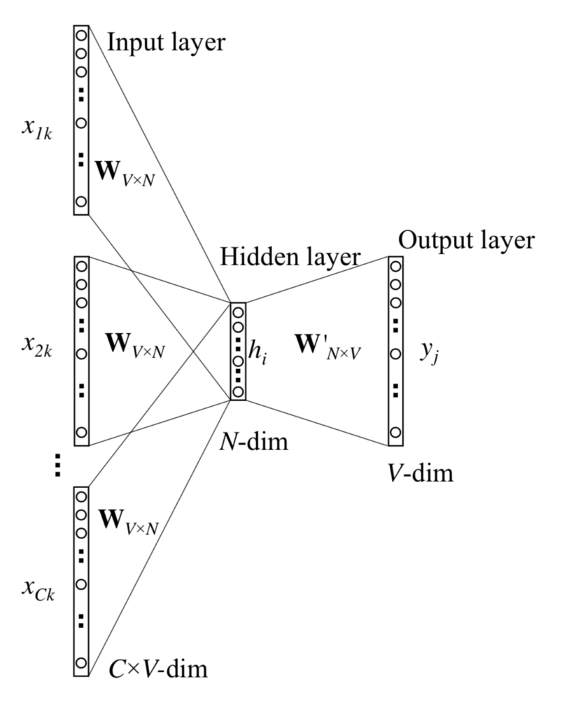
When computing the hidden layer output, instead of directly copying the input vector of the input context word, the CBOW model now takes the average of the vectors of the input context words, and use the product of the input $\rightarrow$ hidden weight matrix and the average vector as the output.

$\begin{equation*} \mathbf{h} = \frac{1}{C}\mathbf{W}^T(\mathbf{x}_1 + \mathbf{x}_2 + \cdots + \mathbf{x}_C) = \frac{1}{C}(\mathbf{v}_{x_1} + \mathbf{v}_{x_2} + \cdots + \mathbf{v}_{x_C})^T \end{equation*}$

where $C$ is the number of words in the context, $x_1, \cdots , x_C$ are the words in the context, and $\mathbf{v}_x$ is the input vector of a word $x$ .

Skip-Gram Model

The Skip-Gram model is the opposite of the Multi-Word CBOW model. The target word is now at the input layer, and the context words are in the output layer.

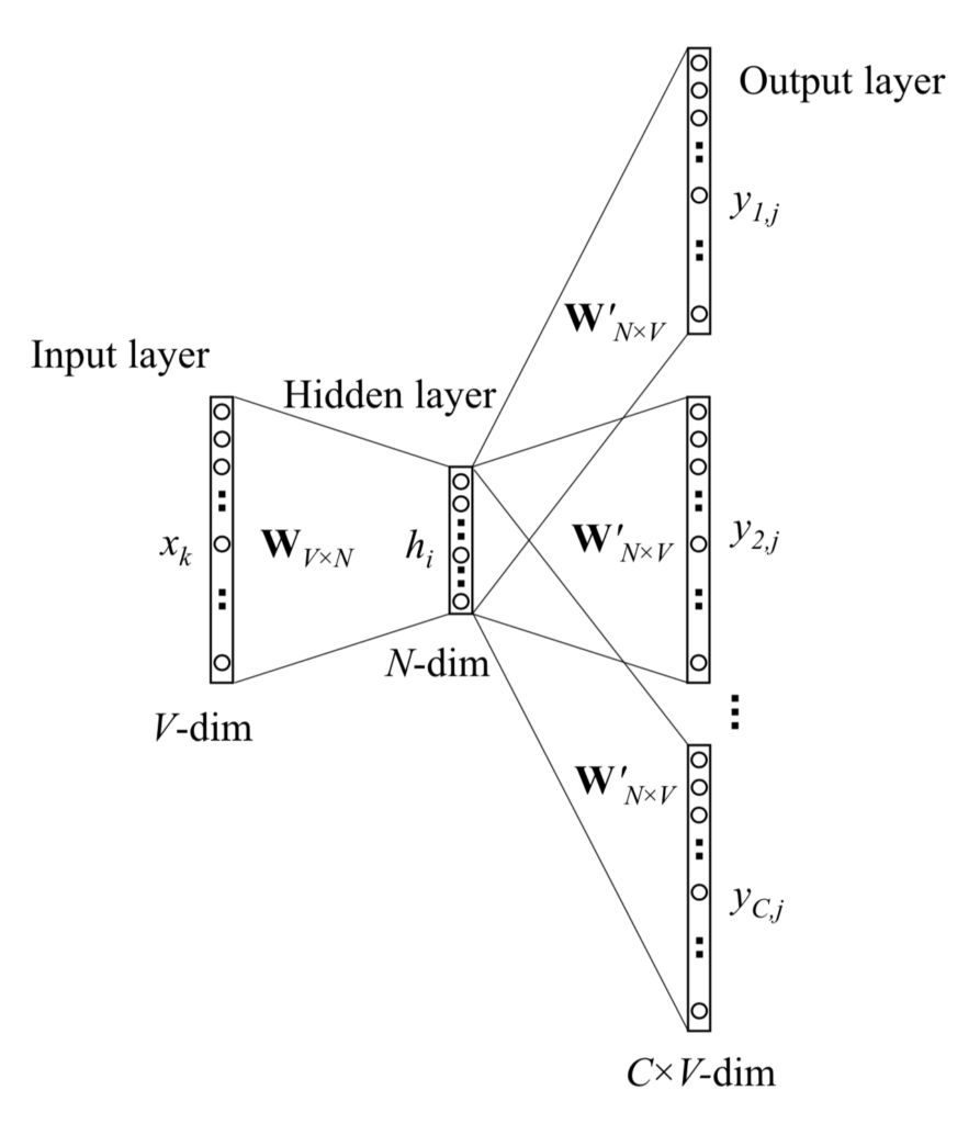
On the output layer, instead of outputing one multinomial distribution, there are $C$ multinomial distributions. Each output is computed using the same hidden $\rightarrow$ output matrix

$\begin{equation*} p(x_{c,j} = x_{O,c}|x_{k}) = y_{c,j} = \frac{\text{exp}(u_{c,j})}{\sum_{j'=1}^V\text{exp}(u_{j'})} \end{equation*}$

where $x_{c,j}$ is the $j$ -th word on the $c$ -th panel of the output layer; $x_{O,c}$ is the actual $c$ -th word in the output context words; $x_i$ is the only input word; $y_{c,j}$ is the output of the $j$ -th unit on the $c$ -th panel of the output layer; $u_{c,j}$ is the net input of the $j$ -th unit on the $c$ -th panel of the output layer. Because the output layer panels share the same weights,

$\begin{equation*} u_{c,j} = u_j = \mathbf{v}_{x_{j}}^T \cdot \mathbf{h}, \quad \quad \text{for } c \in \{1, 2, \cdots ,C \}. \end{equation*}$

where $\mathbf{v}_{x{j}}$ is the output vector of the $j$ -th word in the vocabulary, $x_j$ , and also $\mathbf{v}_{x{j}}$ is taken from a column of the hidden $\rightarrow$ output weight matrix, $\mathbf{W}'$ .

References

https://arxiv.org/pdf/1411.2738.pdf

The Beard Sage