Hidden Markov Models Likelihood Computation - The Forward Algorithm

Computing Likelihood

Given an Hidden Markov Model defined by $\lambda = (A, B)$ and an observation sequence $O$ , determine the likelihood that the observation sequence was generated by this model, $P(O|\lambda)$ .

For a particular hidden state sequence $Q = q_1,q_2,\cdots,q_T$ and an observation sequence $O = o_1,o_2,\cdots,o_T$ , the likelihood of the observation sequence is defined as

$\begin{equation*} \begin{split} & P(O|Q,\lambda) \\ =\, & P(o_1,o_2,\cdots,o_T|q_1,q_2,\cdots,q_T,\lambda) \\ =\, & P(o_1|o_2,\cdots,o_T,q_1,q_2,\cdots,q_T,\lambda)P(o_2,\cdots,o_T|q_1,q_2,\cdots,q_T,\lambda) \\ = & P(o_1|q_1,\lambda)P(o_2,\cdots,o_T|q_1,q_2,\cdots,q_T,\lambda) \\ =\, & P(o_1|q_1,\lambda)P(o_2|o_3,\cdots,o_T,q_1,q_2,\cdots,q_T,\lambda)P(o_3,\cdots,o_T|q_0,q_1,q_2,\cdots,q_T,\lambda) \\ =\, & P(o_1|q_1,\lambda)P(o_2|q_2,\lambda)P(o_3,\cdots,o_T|q_1,q_2,\cdots,q_T,\lambda) \\ \,& \vdots \\ =\, & \prod_{i=1}^{T}P(o_i|q_i,\lambda) \end{split} \end{equation*}$

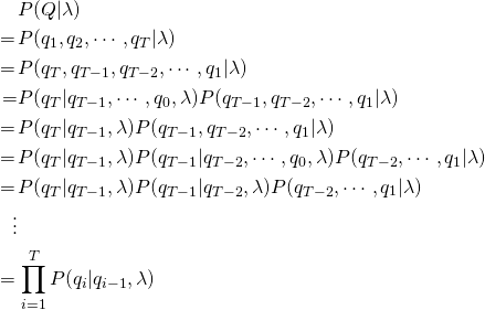
The likelihood of the state sequence is defined as follows. The start state is excluded for now and added at the end.

$\begin{equation*} \begin{split} & P(Q|\lambda) \\ =\, & P(q_1,q_2,\cdots,q_T|\lambda) \\ =\, & P(q_T,q_{T-1},q_{T-2},\cdots,q_1|\lambda) \\ = & P(q_T|q_{T-1},\cdots,q_0,\lambda)P(q_{T-1},q_{T-2},\cdots,q_1|\lambda) \\ =\, & P(q_T|q_{T-1},\lambda)P(q_{T-1},q_{T-2},\cdots,q_1|\lambda) \\ =\, & P(q_T|q_{T-1},\lambda)P(q_{T-1}|q_{T-2},\cdots,q_0,\lambda)P(q_{T-2},\cdots,q_1|\lambda) \\ =\, & P(q_T|q_{T-1},\lambda)P(q_{T-1}|q_{T-2},\lambda)P(q_{T-2},\cdots,q_1|\lambda) \,& \vdots \\ =\, & \prod_{i=1}^{T}P(q_i|q_{i-1},\lambda) \end{split} \end{equation*}$

where $q_0$ is the same as the start state $q_s$ .

Combining the two results above

$\begin{equation*} P(O,Q|\lambda) = P(O|Q, \lambda) \cdot P(Q|\lambda) = \prod_{i=1}^{T}P(o_i|q_i,\lambda) \cdot \prod_{i=1}^{T}P(q_i|q_{i-1},\lambda) \end{equation*}$

The total probability of the observations can be computed by summing over all possible hidden state sequences

$\begin{equation*} P(O|\lambda) = \sum_{Q}P(O, Q|\lambda) = \sum_{Q}P(O|Q,\lambda)P(Q|\lambda) = \sum_{Q}\Bigg(\prod_{i=1}^{T}P(o_i|q_i,\lambda) \cdot \prod_{i=1}^{T}P(q_i|q_{i-1},\lambda)\Bigg) \end{equation*}$

Time Complexity

A sequence $Q = q_1,q_2,\cdots,q_T$ can have $N^T$ combinations.

Term	Time Complexity
$\sum_Q$	$O(N^T)$
$\prod_{i=1}^{T}P(o_i\|q_i)$	$O(T)$
$\prod_{i=1}^{T}P(q_i\|q_{i-1})$	$O(T)$

Thus the total time complexity will be $O(N^T) \times (O(T) + O(T)) = O(TN^T)$ .

Forward Algorithm

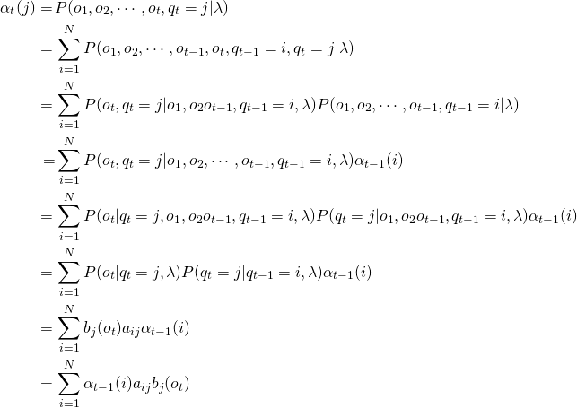
The forward algorithm (a kind of dynamic programming algorithm) is an efficient algorithm, that uses a table to store intermediate values as it builds up the probability of the observation sequence. The forward algorithm computes the observation probability by summing over the probabilities of all possible hidden state paths that could generate the observation sequence, but it does so efficiently by implicitly folding each of these paths into a single forward trellis.

$\alpha_t(j)$ represents the probability of being in state $j$ after seeing the first $t$ observations, given the Hidden Markov Model $\lambda$ . $\alpha_t(j)$ is computed by summing over the probabilities of every path that could lead to this state.

$\begin{equation*} \begin{split} \alpha_t(j) =\, & P(o_1,o_2,\cdots,o_t,q_t=j|\lambda) \\ =\, & \sum_{i=1}^{N}P(o_1,o_2,\cdots,o_{t-1},o_t,q_{t-1}=i,q_t=j|\lambda) \\ =\, & \sum_{i=1}^{N}P(o_t,q_t=j|o_1,o_2…o_{t-1},q_{t-1}=i,\lambda)P(o_1,o_2,\cdots,o_{t-1},q_{t-1}=i|\lambda) \\ = & \sum_{i=1}^{N}P(o_t,q_t=j|o_1,o_2,\cdots,o_{t-1},q_{t-1}=i,\lambda)\alpha_{t-1}(i) \\ =\, & \sum_{i=1}^{N}P(o_t|q_t=j,o_1,o_2…o_{t-1},q_{t-1}=i,\lambda)P(q_t=j|o_1,o_2…o_{t-1},q_{t-1}=i,\lambda)\alpha_{t-1}(i) \\ =\, & \sum_{i=1}^{N}P(o_t|q_t=j,\lambda)P(q_t=j|q_{t-1}=i,\lambda)\alpha_{t-1}(i) \\ =\, & \sum_{i=1}^{N}b_j(o_t)a_{ij}\alpha_{t-1}(i) \\ =\, & \sum_{i=1}^{N}\alpha_{t-1}(i)a_{ij}b_j(o_t) \end{split} \end{equation*}$

where $\alpha_{t-1}(i)$ is the previous forward path probability from the previous time step.

Visualization

Rendered by QuickLaTeX.com

Visualizing the computation of a single element $\alpha_t(j)$ in the trellis by summing all the previous values $\alpha_{t-1}(i)$ , weighted by their transition probabilities $a_{ij}$ , and multiplying by the observation probability $b_j(o_{t})$ . Hidden states are in circles, observations in squares. Shaded nodes are included in the probability computation for $\alpha_t(j)$ .

Initialization

$\begin{equation*} \alpha_1(j) = P(o_1,q_1=j,\lambda) = P(o_1|q_1=j,\lambda)P(q_1=j,\lambda) = a_{sj}b_j(o_1) \quad \quad 1 \leq j \leq N \end{equation*}$

Recursion

$\begin{equation*} \alpha_t(j) = \sum_{i=1}^{N}\alpha_{t-1}(i)a_{ij}b_j(o_t) \quad \quad 1 \leq j \leq N; 1 < t \leq T \end{equation*}$

Termination

$\begin{equation*} P(O|\lambda) = \alpha_{t+1}(q_f) = \sum_{i=1}^{N}\alpha_{T}(i)a_{if} \end{equation*}$

Time Complexity

Initialization step runs in $O(N)$ . Recursion step is run $T \times N$ times and the summation is over $N$ . Thus, the recursion step runs in $O(TN^2)$ . Termination step runs in $O(N)$ . The forward algorithm thus reduces the time complexity to $O(TN^2)$ .